Artistic Style Transfer with Deep Neural Networks
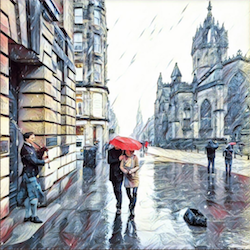
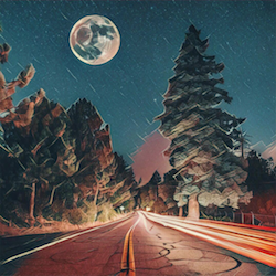
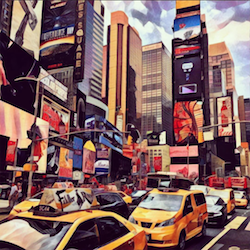
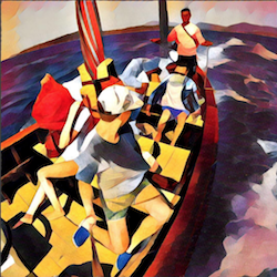
Having recently played with the new Prisma app I was amazed at how seamlessly it is able to apply the style of a particular painting to any image from my camera roll. Some of the photos look like actual works of art! In fact they are works of art - but the artist is no longer a human - it’s an algorithm! Here are a few examples from the Prisma Instagram feed:
It’s no surprise that neural networks are at the heart of this capability. The first major step in this field was introduced in the paper A Neural Algorithm of Artistic Style in September 2015. Gatys et. al show that the task of transferring the style from one image to the content of another can be posed as an optimisation problem which can be solved through training a neural network. In this post I’ll attempt to briefly summarise the main concepts from the paper and share some results I obtained from my own implementation of the algorithm in TensorFlow.
Convolutional neural networks
The most effective neural network architecture for performing object recognition within images is the convolutional neural network. It works by detecting features at larger and larger scales within an image and using non-linear combinations of these feature detections to recognise objects. See my earlier blog post for a more detailed explanation of these networks.
In their paper, Gatys et. al show that if we take a convolutional neural network that has already been trained to recognise objects within images then that network will have developed some internal representations of the content and style contained within a given image. What’s more, these representations will be independent from each other, so we can use the content representation from one image and style representation from another to generate a brand new image.
VGG network
One of the most popular benchmarks for image classification algorithms today is the ImageNet Large Scale Visual Recognition Challenge - where teams compete to create algorithms which classify objects contained within millions images into one of 1,000 different categories. All winning architectures in recent years have been some form of convolutional neural network - with the most recent winners even being able to surpass human level performance!
In 2014, the winner of the ImageNet challenge was a network created by the Visual Geometry Group (VGG) at Oxford University, achieving a classification error rate of only 7.0%. Gatys et. al use this network - which has been trained to be extremely effective at object recognition - as a basis for trying to extract content and style representations from images.
Here’s a diagram of the VGG network:
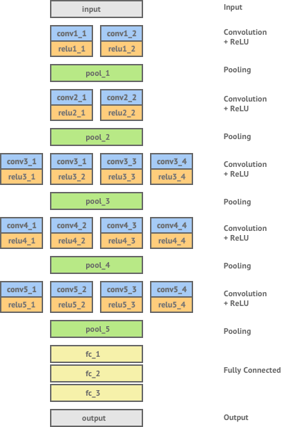
It consists of 16 layers of convolution and ReLU non-linearity, separated by 5 pooling layers and ending in 3 fully connected layers. Let’s see how we can extract representations of the content and style of images from the various layers of this network.
Content representation
The main building blocks of convolutional neural networks are the convolution layers. This is where a set of feature detectors are applied to an image to produce a feature map, which is essentially a filtered version of the image.
Networks that have been trained for the task of object recognition learn which features it is important to extract from an image in order to identify its content. The feature maps in the convolution layers of the network can be seen as the network’s internal representation of the image content. As we go deeper into the network these convolutional layers are able to represent much larger scale features and thus have a higher-level representation of the image content.
We can demonstrate this by constructing images whose feature maps at a chosen convolution layer match the corresponding feature maps of a given content image. We expect the two images to contain the same content - but not necessarily the same texture and style.
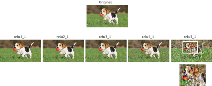
We can see that as we reconstruct the original image from deeper layers we still preserve the high-level content of the original but lose the exact pixel information.
Style representation
Unlike content representation, the style of an image is not well captured by simply looking at the values of a feature map in a convolutional neural network trained for object recognition.
However, Gatys et. al found that we can extract a representation of style by looking at the spatial correlation of the values within a given feature map. Mathematically, this is done by calculating the Gram matrix of a feature map. If the feature map is a matrix , then each entry in the Gram matrix can be given by:
As with the content representation, if we had two images whose feature maps at a given layer produced the same Gram matrix we would expect both images to have the same style, but not necessarily the same content. Applying this to early layers in the network would capture some of the finer textures contained within the image whereas applying this to deeper layers would capture more higher-level elements of the image’s style. Gatys et. al found that the best results were achieved by taking a combination of shallow and deep layers as the style representation for an image.
The diagram below shows images that have been constructed to match the style representation of Pablo Picasso’s ‘Portrait of Dora Maar’. Results are shown for combining an increasing number of layers to represent the image’s style.
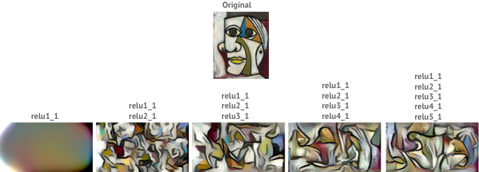
We can see that the best results are achieved by a combination of many different layers from the network, which capture both the finer textures and the larger elements of the original image.
Style transfer as an optimisation problem
Style transfer is the task of generating a new image , whose style is equal to a style image and whose content is equal to a content image . Now that we have a clear definition of the style and content representation of an image we can define a loss function which essentially shows us how far away our generated image is from being a perfect style transfer.
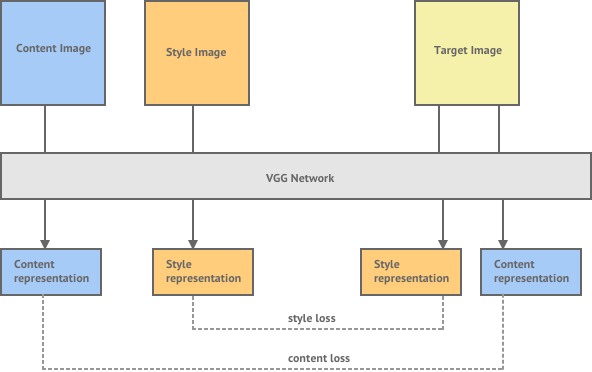
Given a chosen content layer , the content loss is defined as the euclidean distance between the feature map of our content image and the feature map of our generated image . When the content representation of and are exactly the same this loss becomes .
Similarly, given a chosen style layer , the style loss is defined as the euclidean distance between the Gram matrix of the feature map of our style image and the Gram matrix of the feature map of our generated image . When considering multiple style layers we can simply take the sum of the losses at each layer.
The total loss can then be written as a weighted sum of the both the style and content losses, where the weights can be adjusted to preserve more of the style or more of the content.
Performing the task of style transfer can now be reduced to the task of trying to generate an image which minimises the loss function.
Styling an image
The total loss equation lets us know how far we are away from achieving our goal of producing a style transferred image Y. But how do we go about getting there?
To generate a styled image we first start with a random image, sometimes known as white noise. We then iteratively improve the image using a method called gradient descent via backpropagation. The details of this algorithm are best left for another post but if interested you can read more about it here.
To describe it simply, we first pass the image through the VGG network to calculate the total style and content loss. We then send this error back through the network (backpropagation) to allow us to determine the gradient of the loss function with respect to the input image. We can then make a small update to the input image in the negative direction of the gradient which will cause our loss function to decrease in value (gradient descent). We repeat this process until the loss function is below a threshold we are happy with.
Results
Here are some of the best results achieved by Gatys et. al:
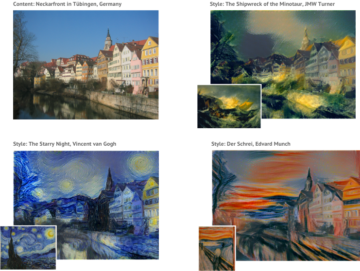
The content image of the Neckarfront in Tübingen, Germany has been styled with four different famous paintings, each producing a very pleasing blend of content and style.
TensorFlow implementation
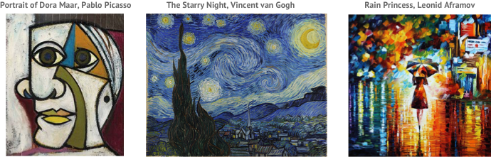
You can find my own TensorFlow implementation of this method of style transfer on my GitHub repository. I generated style transfers using the following three style images:
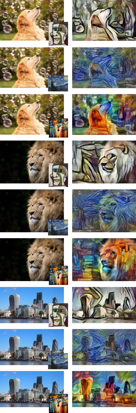
Each optimisation was run for 1000 iterations on a CPU and took approximately 2 hours. Here are some of the style transfers I was able to generate:
If you found this post about style transfer interesting click here to read my next post about performing style transfer in real-time.