Machines that can see: Convolutional Neural Networks

20 Dec 2016

What does it mean to see?

Look at these two images:

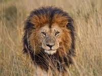
It took you less than 100 milliseconds to identify the first as lion and the second as a tiger.

Your eyes turn the photons from these images into millions of electrical impulses that are fired into the neurons of your brain. Depending on the strength of these electrical signals various neural pathways become activated within the brain. A different set of neural pathways activate when you look at the first image compared to the second, and this is how your brain will interpret one image as a lion and the other as a tiger.

It is not unreasonable to believe that we could train artificial neural networks, which are inspired by the brain, to perform a similar task. They would take image pixels as inputs (instead of electrical signals) and learn to categorise the activations of different neural pathways as lions or tigers, for example.

In fact, image recognition is currently a very popular use of neural networks and in recent years we have seen a vast amount of progress in this field. We’re now able to create machines which can read handwritten text, automatically group and caption images and even drive cars!

In this blog post I hope to briefly outline one of the most successful neural network architectures for image recognition tasks; convolutional neural networks. To motivate the need for convolutional neural networks let’s start by looking at the simplest form of network architecture, which is the fully connected network.

Fully connected networks

A traditional fully connected neural network architecture looks something like this:

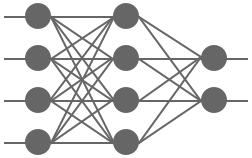
Every neuron in a given layer is connected to every neuron in the following layer, with a weight being assigned to each connection. This network is essentially defining a complex function between the inputs in the first layer and the outputs in the last layer. The weights connecting each neuron are parameters which are tweaked by training the network to learn a specific function, for example to tell whether an image contains a lion or a tiger.

Let’s imagine applying this type of network architecture to our task of image recognition. Assume we have a 50×50 pixel input image and we want to classify it as either a lion or a tiger. Here’s a simple 3 layer network we might want to train:

The input layer has 7,500 neurons - that’s 2,500 pixels each with a red, green and blue component. The hidden layer has 2,000 neurons and the output layer has 2 neurons - one for lions and the other for tigers. So what’s the total number of connections in this network?

(7,500 × 2,000) + (2,000 × 2) = 15,004,000

The number of weights we would need to learn for this network is approximately 15 million! We would need a large amount of training data and a lot of computing power to even begin to train it effectively.

Given these practical considerations, a different architecture called convolutional neural networks have become much more popular for image recognition tasks. They work by detecting patterns at various scales within an image and using these to identify objects within the image. Significantly, they require many orders of magnitude less weights to train and as a result have become the standard.

Convolutional neural networks

Here’s an example of a convolutional neural network:

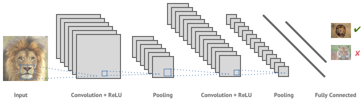
It consists of a number of layers of convolution, non-linearity and pooling, followed by a final set of fully connected layers. Let’s break down each of these types of layers.

Convolution

The main building blocks of convolutional neural networks are the convolution layers, which are used to detect the presence of features within an image. Features could be anything from simple edges and curves to more complex structures like ears, noses and eyes.

A convolution layer is created by defining a kernel - which is fixed square window of weights, and scanning this across the whole input image.

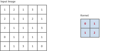
At each location in the image it performs a convolution operation on the image pixels within the kernel window and the kernel weights. This is simply the total sum of the pixel values within the kernel window multiplied by the corresponding kernel weight.

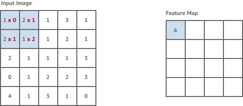
The convolution operation is essentially trying to detect the presence of a feature within the kernel window. The type of feature that it’s looking for is determined by the values of the kernel weights. The resulting output is called a feature map, which describes the presence of a given feature throughout the input image. As an example, applying a kernel which detects edges to our tiger image results in the following feature map:

To perform image recognition it is necessary to consider many different types of features in combination with each other and so a single convolutional layer will typically contain many different feature maps. Note that we don’t need to specify beforehand what types of features our kernels will be looking for. As we train the network we will adjust the weights of the kernels to improve the accuracy of the network and so the network will decide which features are important to detect.

Finally, we can also get an intuition for the number of weights we need to learn when training a a convolutional neural network Let’s imagine we have 4 convolutional layers, each with 64 feature maps that each have a 3×3 kernel window. The number of weights in the network is then:

(3 × 3) × 64 × 4 = 2,304

Which is drastically smaller than the 15 million weights we required to train our fully connected network earlier!

Non-linearity (ReLU)

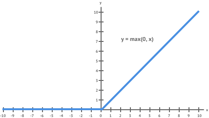
Neural networks attempt to learn a function by taking a combination of all of the functions at each stage in the network. Convolution is a linear operation, so combining many convolution layers will still only allow us to learn a linear function. This unfortunately is not adequate for most real-world tasks we would want to solve, including our example of image recognition. In order to allow our network to learn more complex non-linear functions we need to introduce some non-linearity.

In convolutional neural networks this is done by applying a non-linear function to each of the feature maps produced in the convolution layers. The most common non-linear function used is the rectified linear unit (ReLU) shown below. It is an element-wise operation which replaces negative values with 0. It’s one of the most widely used non-linear functions in neural networks because it has some nice properties which help to avoid problems such a gradient saturation during training.

Pooling

Feature maps give us a detailed picture of where specific features occur within an input image. For image recognition tasks we don’t always need to know the exact pixel locations of the features we detect. For example, if our tiger image was shifted slightly to the right - it would still be an image of a tiger, even if it’s eyes and ears and mouth are now a few pixels across. The pooling operation helps to introduce this desired positional invariance into our networks.

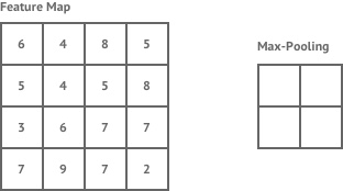
Pooling layers are a form of downsampling which usually follow convolution layers in the neural network. Applying pooling to a feature map transforms the map into a smaller representation, and it loses some of the exact positional information of the features. Therefore it makes our network more invariant to small transformations and distortions in the input image by asking whether a feature appears in a given region of an image (the pooling region) rather than at a specific location.

The most common method of pooling is max-pooling, where the the maximum value of a given region in a feature map is taken. The example below shows max pooling being applied with a 2×2 pooling region.

Higher Level Features

As a convolutional neural network gets deeper the feature maps in the convolution layers are able to pick out more and more complex features.

Whereas in the earlier layers, feature maps may be detecting simple structures such as horizontal or vertical edges, feature maps in deeper layers may be looking for more complex structures like eyes, ears or mouths.

Why is this? It can be explained by the concept of the receptive field of a kernel filter. In the first convolution layer, a 2×2 kernel only has access to 4 pixels from the input image - so it wouldn’t be possible for this filter to detect ears, but it could accurately detect transitions from light to dark (i.e. edges).

After a 2×2 pooling layer, each element in the pooled feature map is influenced by 4 pixels from the original input image. The 2×2 kernel in the next convolution layer will now be influenced by 16 pixels from the input image. As the convolution layers get deeper each kernel is able to “see” a much large part of the input image and can therefore detect more complex features. This is why as a convolutional neural network grows larger we are able to detect much larger structures, eventually allowing us to classify lions and tigers.

Fully Connected layer

Most convolutional neural networks end with one or more fully connected layers. This allows the network to learn a function which maps the final layer of high-level feature maps to each of the image classifications. For example, if my image contains two eyes, a nose, sharp teeth and a body with stripes I may be very confident that it’s a picture of a tiger.

From Bits to Brains