Style Transfer in Real-Time
In my previous post I discussed the goal of transferring the style of one image onto the content of another. I gave an outline of the paper A Neural Algorithm of Artistic Style which formulated this task as an optimisation problem that could be solved using gradient descent. One of the drawbacks to this approach is the time taken to generate styled images. For each style transfer that we want to generate we need to solve a new optimisation problem. Each of the following style transfers took approximately 2 hours to generate using a CPU and running for 1000 iterations:
So how do apps such as Prisma allow users to apply different styles to a content image and run this on the CPU of a mobile device within seconds rather than hours?
Real-time style transfer
In March 2016 a group of researchers from Stanford University published a paper which outlined a method for achieving real-time style transfer. They were able to train a neural network to apply a single style to any given content image. Given this ability, a different network could be trained for each different style we wish to apply.
The paper, titled Perceptual Losses for Real-Time Style Transfer and Super-Resolution by Johnson et. al, shows that it is possible to train a neural network to apply a single style to any given content image with a single forward pass through the network.
In this post I’ll give an overview of the method they propose and share some results I obtained from my own implementation in TensorFlow.
Learning to optimise
The original algorithm proposed by Gatys et. al formulated a loss function for style transfer and reduced the problem down to one of optimising this loss function. Johnson et. al show that, if we limit ourselves to a single style image, we can train a neural network to solve this optimisation problem for us in real-time and transform any given content image into a styled version.
The diagram below gives an overview of the system they propose:
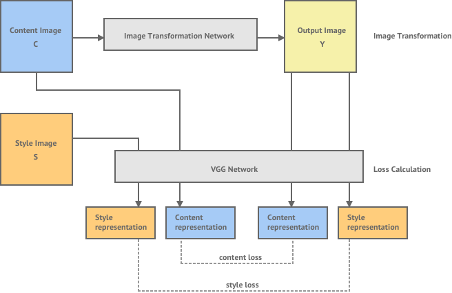
This system consists of both an image transformation network and a loss calculation network. The image transformation network is a multi-layer convolutional neural network that will transform an input content image into an output image , where should have the content of the content image and the style of a separate style image .
The loss network is used to calculate a loss between our generated output image and our desired content and style images. We calculate loss in the same way as the previous method, by evaluating the content representation of and the style representation of and taking the distance between these and the content and style representations of our output image . These representations are calculated using the VGG network, which is a network that has be pre-trained for object recognition. You can read a more detailed explanation of the style transfer loss function in my earlier post.
Given this system, we can then train the image transformation network to reduce the total style transfer loss. To train the network, we pick a fixed style image and use a large batch of different content images as training examples. In their paper, Johnson et. al trained their network on the Microsoft COCO dataset - which is an object recognition dataset of 80,000 different images.
Training involves using the loss network to evaluate the loss for a given training example and then propagating this error back through every layer in the image transformation network. At each layer we compute the gradient of the layer’s weights with respect to the loss function and use this to make a small adjustment to the weights in the negative direction of the gradient. This will iteratively improve the performance of the network until the loss is below an acceptable threshold. This technique is known as gradient descent via backpropagation and iteratively improves the network weights to reduce the value of the loss function. You can read more about it here.
Image transformation network
The diagram below shows the architecture for the image transformation network laid out by Johnson et. al:
![]()
It consists of 3 layers of convolution and ReLU non-linearity, 5 residual blocks, 3 transpose convolutional layers and finally a non-linear tanh layer which produces an output image. Let’s briefly describe what each of these layers are doing.
Downsampling with strided convolution
Convolution layers are used to apply filters to an input image. This is done by moving a fixed-size kernel filter across the input image and applying the convolution operation to the pixels within the kernel window to compute each corresponding pixel in the output image. By default, after each convolution operation we move the kernel window across by 1 pixel. This is known as stride 1 convolution.
If the input image has size pixels, stride 1 convolution with a kernel size generates an output image of size:
This is slightly less resolution than our original input image. If we wish to maintain exactly the same resolution we can use a strategy called zero padding, which adds layers of zero-valued pixels around the input image so that the output is still pixels.
The first convolution layer in our network is stride 1 but the following two layers are stride 2. This means that each time we move the kernel it is shifted by 2 pixels instead of 1, and our output images are now of size
Stride 2 has the effect of halving the size of the input image, which is known as downsampling.
The main reason for including downsampling layers in a convolutional neural network is to increase the receptive field size of the kernel filter in the layers that follow. As the input image becomes downsampled each pixel in that input will be the result of a calculation involving a larger number of pixels from the original input image. In a sense this will allow kernel filters to have access to a much larger part of the original input image without having to increase the kernel size. The reason this is desirable is because style transfer involves applying a given style to an entire image in a coherent way, and so the more information each filter has about the original input image the more coherently our network can apply the style.
An alternative way to introduce downsampling in this convolution neural network would have been through a pooling layer which also reduces the image size.
Upsampling with fractionally strided convolution
After applying both stride 2 convolution layers our image resolution is reduced to of it’s original size. The desired output of our transformation network is a styled image with the same resolution as the original content image. In order to achieve this we introduce two convolution layers with stride . These are sometimes referred to as transpose convolution layers or deconvolution layers. These layers have the effect of increasing the output image size, which is known as upsampling.
Convolution with stride involves moving the kernel window across by half a pixel each time. This results in an output image that has double the resolution of the input. In reality we can’t actually move our kernel along by half a pixel, so instead we pad the existing pixels with zero-valued pixels and carry out a normal stride 1 convolution as shown below.
This achieves the same effect of double the image resolution and results in the final image being the same resolution as our original input image.
Residual layers
Between the downsampling and upsampling layers we have 5 residual layers. These are stride 1 convolution layers but the difference between these and normal convolution layers is that we add the input of the network back to the generated output.
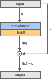
The reason for using residual layers in a network is that for certain tasks it makes it easier to train the network because it has less work to do. Our layer doesn’t need to learn how to take our input and generate a new output - but instead it just needs to learn how to adjust our input to produce our output. They are called residual layers because we are just trying to learn the difference, or residual, between our input and our desired output.
For a task like style transfer using residual layers makes sense as we know that our generated output image should be somewhat similar to our input image so we can help the network by only requiring it to learn the residual.
Constraining the output with a tanh layer
In order to process an image in a neural network it is first represented as a matrix of integers which are the values of each pixel in the image. These have a range of 0 to 255. Each layer in a neural network performs a mathematical operation on its input to produce an output and there is no inherent constraint in these layers that keeps the output bounded between 0 and 255.
After our final layer we want to produce a valid image as this is the final result of our style transfer. This means the generated output must contain values that are all in the valid pixel range of 0 to 255. To achieve this we introduce a final non-linear layer which applies a scaled function to each element in the output.
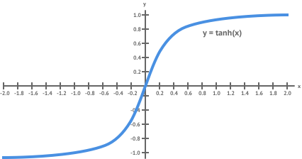
The function is bound between -1 and 1 so by applying this and rescaling the result we can constrain our generated image to have valid pixel values.
Results
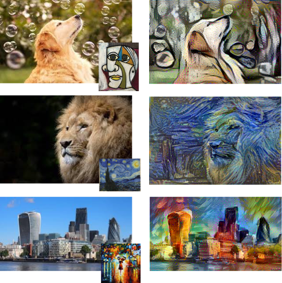
Here is a sample of some of the results achieved by Johnson et. al:
The image transformation networks were trained on 80,000 training images taken from the Microsoft COCO dataset and resized to 256×256 pixels. Training was carried out for 40,000 iterations with a batch size of 4. On a GTX Titan X GPU training each network took approximately 4 hours and image generation took 15 milliseconds on average.
TensorFlow implementation
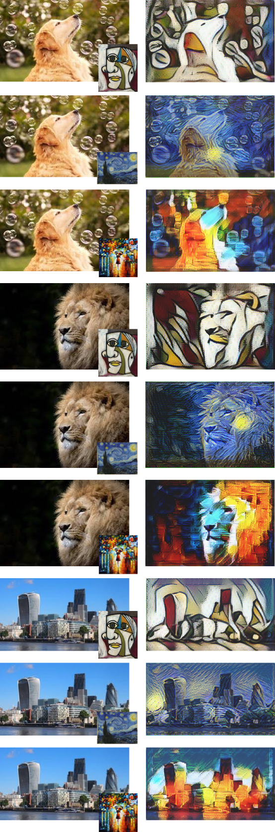
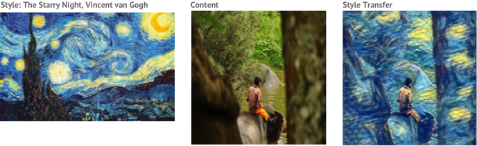
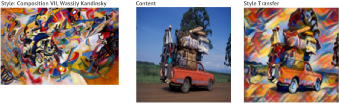
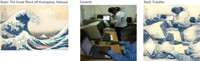
You can find my own TensorFlow implementation of real-time style transfer here. I trained three networks on the following three style images:
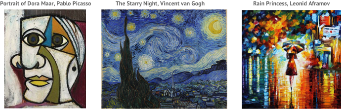
Each network was trained with 80,000 training images taken from the Microsoft COCO dataset and resized to 256×256 pixels. Training was carried out for 100,000 iterations with a batch size of 4 and took approximately 12 hours on a GTX 1080 GPU.
Using the trained networks to generate style transfers took only 5 seconds on a CPU. Here are some of the images I was able to generate: